Previously, we announced alpha support for vector indexes in Dolt. Vector indexes are the new hotness in SQL databases, with recent projects like MariaDB Vector, sqlite-vec, and pgvector adding vectors to popular SQL engines. So naturally, we wanted Dolt to support vectors too.

But this isn't just about staying up to date with these other projects, because Dolt isn't just a SQL engine. It's a version controlled database, and as far as we know, the only version controlled SQL database. And in our six years of adding features, we've made two key observations:

• Making new features work with version control often requires novel data structures and algorithms.
• Adding version control to other features often unlocks capabilities that neither feature can accomplish alone.

And this held true when it came to vector support: version control plus vector indexes turned out to be more than the sum of its parts.

Dolt's big leg up in the vector space is that can efficiently store multiple versions of vector embeddings, reusing storage space for the embeddings that exist in both versions. This is similar both in concept and in implementation to how HuggingFace efficiently stores version-controlled Parquet files, but with two very important bonuses: while Parquet is a serialization format, Dolt is both live and indexed. It's not just the underlying data that's deduplicated, but the indexes as well. And let's us do some pretty awesome things:

• Dolt can store snapshots of a knowledge base at different moments in time, allowing for easy comparison of both the datasets and the results of using them in queries. No rebuilding or updating of the index is necessary.
• If the result of a search changes unexpectedly, Dolt makes it easy to roll back the database to restore the original behavior, and then diff the branches to find out exactly what changed and why.
• It's possible to use branches to explore changes to the dataset before merging those changes back into a main branch, without the time and storage cost of maintaining a separate index.

Today I wanted to explore how exactly we accomplished this. We gave a high-level overview before, but I wanted to do a deeper dive into the novel algorithm work that made this possible, both because it's fascinating, and because it suggests opportunities for future work in this space.

Overview: What is a Vector Index

Feel free to skip ahead to the next section if you already know this; it's mostly a recap from our previous blog post on the topic.

A vector index is a precomputed data structure designed for optimizing an "approximate nearest neighbors search" for a multidimensional vector column. You can imagine vector indexes as a generalization of spatial indexes (which Dolt already supports) onto higher dimensions, but optimized specifically for a single type of search.

It's "approximate" because if the query is to find the N closest neighbors to some vector, it's okay if the result isn't exactly the N closest neighbors, we're allowed to miss some in the name of speed.

The accuracy of an index is called its "recall." Higher recall is better, but it's not the most important factor.

The Need for Novelty

There are already two well-established algorithms for vector indexes: Hierarchical Navigable Small World Graphs (HNSW) and Inverted File Indexes (IVF). So why did we invent our own approach instead of just using one of these?

The problem is that in both of these algorithms, the structure depends on both the order that the vectors were inserted into the dataset, and when the index was initially created. This means that branches that contain the same data might have indexes that look very different, depending on the sequence of operations that happened in each branch. This hampers our ability to efficiently store each version of the index, as well as our ability to predictably merge changes. In order to get these desired properties, the index data structure needs to have a trait known as history independence, which essentially means that the shape of the index is uniquely determined by the data it currently stores, not its operation history. Current vector indexes simply don't provide this feature.

Approaching this from another angle, why couldn't we just reuse Dolt's existing index data structure for vectors? We covered this in a previous blog, but the core problem is that while Dolt's typical indexes have history dependence, they lack spacial locality: a vector index requires that vectors that are close in the vector space are close in the index as well. Normal indexes impose an ordering on the set elements, but trying to map a multi-dimensional vector space onto a one-dimensional ordering is inevitably going to lead to situations where similar vectors appear very far apart in the index.

We need an approach that gives us both properties: clustering vectors based on spacial locality, while also ensuring that this clustering happens in a history-independent manner, without needing to rebuild the index after every operation.

To achieve this, we designed a hybrid approach that combined aspects of both HNSW and IVF with Prolly Trees, the data structure that Dolt uses to achieve history independence. The result is a novel tree structure that our codebase currently calls a Proximity Map.

The Structure of a Proximity Map

The Proximity Map structure most closely resembles a hierarchical IVF index: vectors are divided into buckets, and for each bucket we choose a representative vector such that every vector is closer to its own bucket's representative than it is to any adjacent¹ bucket's representative. Then we apply this process recursively to the representative vectors, putting them into their own buckets with their own representatives. We repeat this process, with each iteration having a fraction of the number of vectors from the previous generation, until we reach a point where every remaining vector is placed in the same bucket.

We then store this data structure as a Merkle tree, where each node in the tree corresponds to one of these buckets, and each level of the tree corresponds to an iteration of this process. The final iteration, with its single bucket, becomes the root of the tree. Each node contains the vectors of its corresponding bucket, and maps each of those vectors onto the child node for which that vector is the representative.

This is best illustrated by an example. For a small set of two-dimensional vectors, a valid proximity map might look like this:

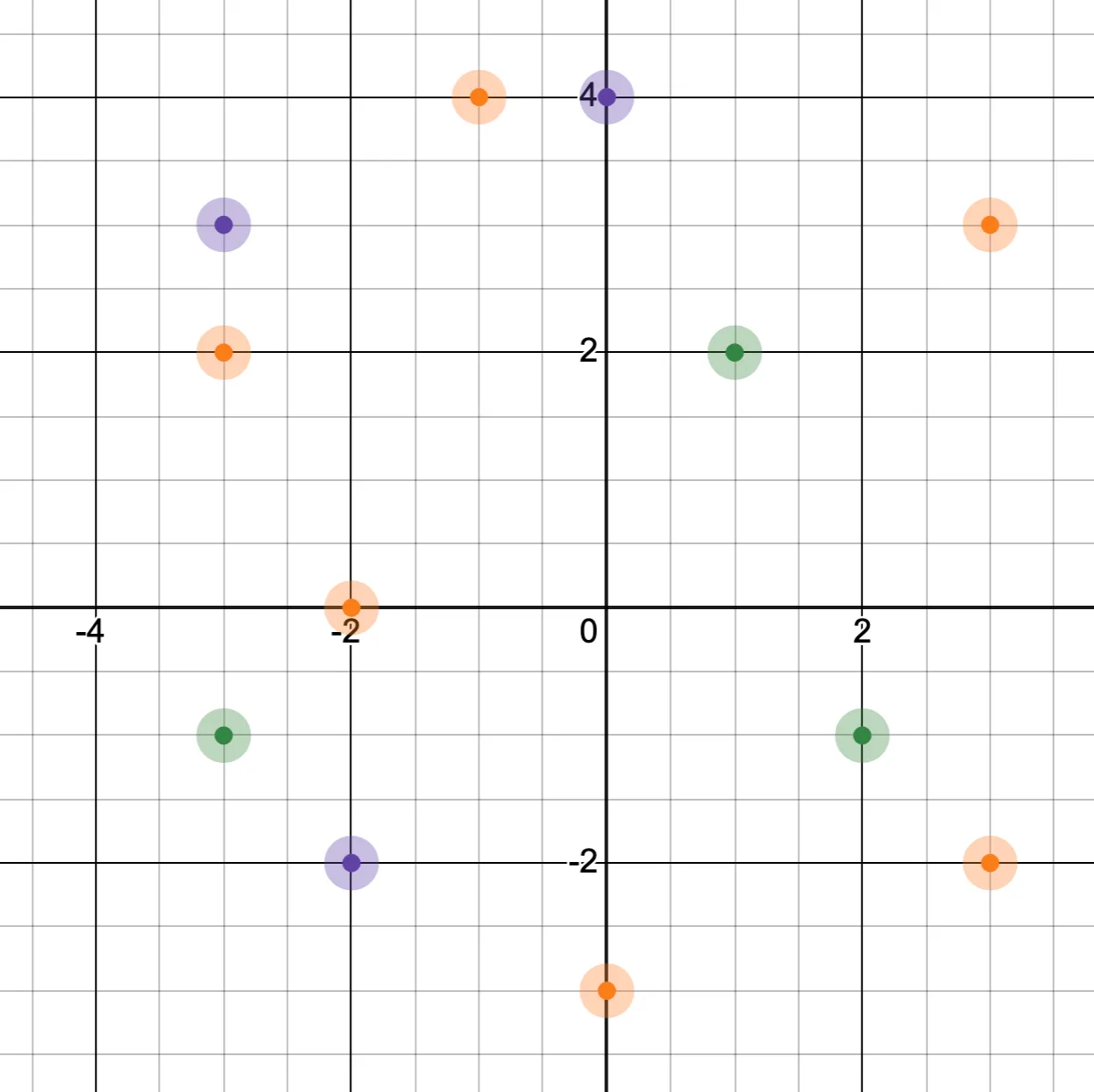
I've color-coded each vector according to the highest level in which it appears.

Note that real vector indexes contain more than just vectors. Real vector indexes store key-value pairs, where the vector makes up part of the key. This allows for additional data to be stored alongside the vector, which is much more useful. But for simplicity, we'll assume for these examples that only vector data is being stored. Real vector indexes also usually have way more than two dimensions, but 2D is a lot easier to visualize.

We also have a notion of the vector path of a node, which is the sequence of vectors used to reach a given node from the root. In this example, the vector path to reach [-1, +4] would be the sequence [+1, +2] -> [0, +4] -> [-1, +4].

Proximity Maps have two important invariants:

• If a vector appears in a non-leaf node, it also appears in the child node that vector maps to. This means that if a vector appears in a non-leaf node, then there's a path of connected nodes from there to the leaf that also contains that vector.
• If a vector V appears in a non-root node N, then for each node between N and the root, it is required that V is closer to the vector that appears in N's vector path than to any other vector in that node.

This is what we meant when we talked about "adjacent" buckets earlier: each node partitions the vector space, and the node's children partition that space further. In this example, Node₀₁ is "adjacent" to its sibling, Node₀₀, but not Node₁₀.

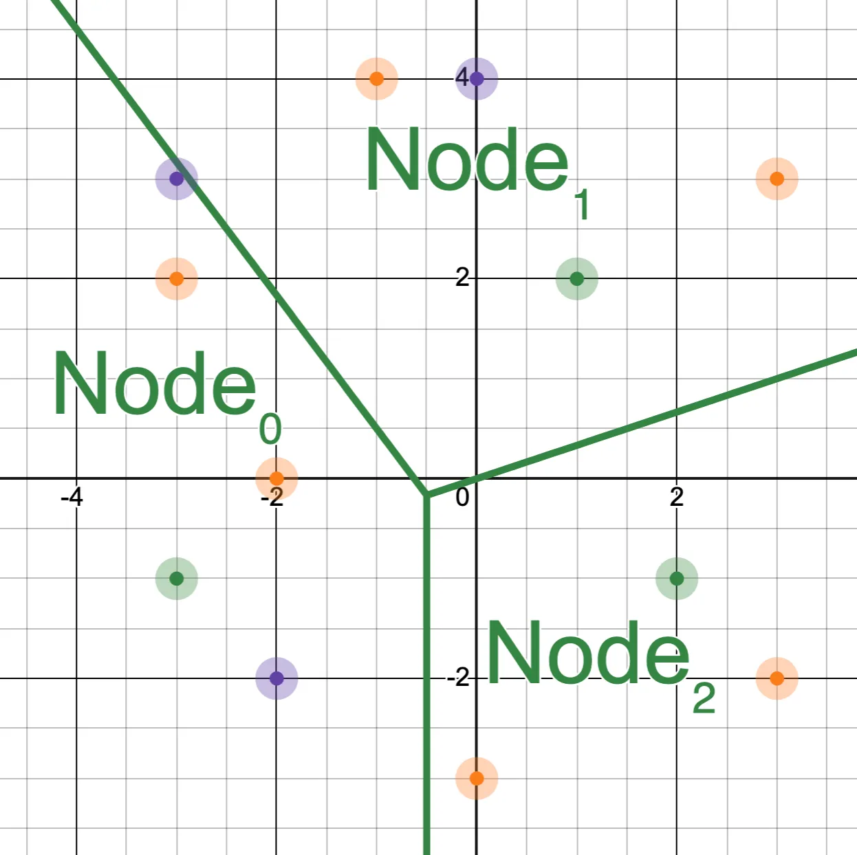
The best way to think of this is to realize that each node represents a specific region of the vector space, where each node's children subdivide the space of the parent. The vectors that appear in the root node partition the space according to the Voronoi diagram of those points:

And the vectors that appear one level deep partition each of those regions:

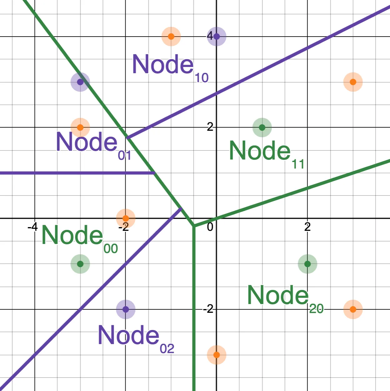
These graphs visualize an important consequence of the invariants: every vector appears in the partition defined by all of its parent nodes.

But there's one important detail we've been glossing over: how do we choose the representative vectors at each level? Recall that we're trying to achieve history-independence: the choice of representatives needs to be purely a function of the vectors in the dataset. We also want incremental changes like adding and removing vectors to be as efficient as possible, so adding a removing a vector shouldn't change any representatives other than the added or removed vector.

If you've read our other blog posts about Prolly Trees, this should start to sound very similar to how Prolly Trees need to determine "chunk boundaries", the key values that demarcate the end of one node and the start of another. And we adopt a similar solution here. Specifically, we draw inspiration from the same paper that guided BlueSky's Prolly Tree implementation, which I touched on in my last blog post. The idea is to hash each index key (in this case, our vector), and calculate a "max level" for the key based on the number of leading zeroes in the hash. This will the highest level where that key appears in the tree. So if we show the binary hashes alongside the keys, it might look like this:

By adjusting the number of leading zeros required to reach a new level in the tree, we can control the average size of each node. For this example, you can see that each level has 1 more leading zero than the previous level, leading to an average node size of 2¹ = 2.

In practice, we chose 8 leading bits per level, leading to an average node size of 2⁸ = 256 vectors. This was chosen somewhat arbitrarily, mainly because we wanted to minimize the probability that a node exceeded 16KB in practice. Some experimentation suggested that 8 bits per level was suitable for this.

There are some downsides to determining max levels this way, the biggest one being that it leads to a geometric distribution of node sizes. Geometric distribution of node sizes can cause suboptimal performance in the worst case: a node that is larger is not only slower to use in a lookup, but is also more likely to be used in a lookup because it contains more vectors than a smaller node. But there are upsides to this approach as well: the vectors that appear in each level is a uniform sampling of the total dataset, preserving any trends or distribution patterns in the underlying data.

We predict that the process of choosing max levels for vectors and/or other ways to determine the shape of the tree will be an area of active research.

Performing an Approximate Nearest Neighbors Search

The algorithm for performing an Approximate Nearest Neighbors Search on a Proximity Map very similar to lookup functions on other existing vector indexes:

1. To find the N closest vectors to some target vector V, pick some buffer size M > N.
2. Starting with the root node, identify the M vectors that are closest to the target vector. These are the current candidates.
3. Recurse into the next level of the tree, only looking at the buckets that contain the current candidates. From among those buckets, find the M vectors that are closest to the target.
4. Continue this process until we reach the leaf nodes.
5. Finally, of the M candidates, find the N that are closest to the target and return those.

Picking a larger value for M increases the runtime and memory requirements of the lookup, but results in higher recall. As previously mentioned, recall is a measurement of vector indexes that indicates the rate of false negatives: the number of vectors that aren't returned by a lookup despite being close to the target. A higher recall means less false negatives. Vector indexes never return false positives, only false negatives.

Let's look at an example where a false negative can occur, and see how increasing the candidate size can prevent it. In our example above, suppose we want to find the single vector that's closest to [-2, +3]. If we pick M = 1, then at each level of the tree we track only the single closest candidate.

Here's a visualization of the tree, where at every level, the vectors that make up the candidate set are green, the non-candidate vectors visited during the traversal are yellow, and vectors not visited are red:

The lookup would return [-1, +4] as the closest vector. But the actual closest vector is actually [-3, +3], with a distance of 1.00 compared to 1.41.

But if we pick M = 2, the same visualization looks like this:

Because [-3, +3] appears in the final buffer, we correctly identify it as the closest vector in the index.

This shows how setting the size of the candidate set to be larger than the number of requested matches allows for good recall even when results fall in different buckets.

Building a Proximity Map

We've seen how a proximity map can be used in a nearest neighbor's search, but not how to create such a data structure. Building a proximity map that has the desired properties has an issue: before we can determine which vectors are in a node, we must determine all of the vectors in its parent node. This presents two challenges:

1. We cannot simply stream the data and build the tree as we go, like we do when building traditional Prolly Trees. Instead, we must go in multiple passes: one pass to determine the level of each vector, and at least one additional pass to build the tree. This necessarily requires O(N) space as well to store the shape of the tree.
2. This necessitates that we build the tree from the root to the leaves. But our end goal is create a Merkle tree. In a Merkle tree, each node contains the content-addressed hash of its children, which necessitates that we build the tree from the leaves to the root. So we'll also need a way to represent intermediate results before we're able to write leaf nodes.

Essentially, we need to: a. Determine and store the shape of each level, starting from the root and ending at the leaves. b. Build the nodes, starting at the leaves and ending at the root.

This necessarily requires O(N) space to store the shape of the non-leaf nodes.

In order to accomplish this in a real application without using unbounded memory, we need to be able to flush these intermediate data structures to disk, even as we're still building them, then read back individual elements only as we need them.

In most contexts, this is a nontrivial task. But here's the lucky break: We're adding this algorithm to a database engine. And these storage requirements just so happen to be what relational database primitives already do. We can take advantage of that.

In order to build the final tree structure, Dolt applies a series of transformations to intermediate ordered maps, each of which is built from the same primitives that Dolt uses to create database tables. As a result, these maps get automatically get flushed to disk in order to constrain memory. It was a surprisingly elegant way to implement an algorithm.

You can find the code in go/store/prolly/proximity_map.go, and I'll go over it at a high level here.

Note: when talking about tree levels, we typically count from the leaves (leaf nodes are level 0, their parents are level 1, etc.) But sometimes it's more helpful to count from the root. We use the term "depth" when counting from the root, and "level" when counting from the leaves. So for example, in a tree with 5 levels, the root is level 4 (and depth 0), while the leaves are level 0 (and depth 4).

The process works in stages:

Step 1: Create levelMap, an ordered map of (indexLevel, key) -> value

Here, indexLevel is the maximum level in which the vector appears, sorted in decreasing order. key is a byte sequence containing the index key (which includes the vector, or for larger vectors a content-addressed hash). And values is the value of the index row, if any (in our example, we don't have any value data, so we omit this).

Building this from the table is easy: for each table row, hash the key, compute the level from the number of leading zeroes, and insert it into the ordered map.

For our example, after inserting every row into the levelMap, it looks like this:

Max Level	Key
2	[-3, -1]
2	[+1, +2]
2	[+2, -1]
1	[-3, +3]
1	[-2, -2]
1	[0, +4]
0	[-3, +2]
0	[-2, 0]
0	[-1, +4]
0	[0, -3]
0	[+3, -2]
0	[+3, +3]

Step 2: Create pathMaps, a list of maps, each corresponding to a different depth of the ProximityMap

The pathMap for a given depth contains an entry for every vector that appears at that depth, and is built using the data from the previous pathMap, starting at the root and working toward the leaves. These maps must be built in order, from shallowest to deepest.

The pathMap at depth i has the schema (vectorPath, key) -> value, where vectorPath is the sequence of vectors visited when walking the tree from the root to the key at the current depth. key and value retain their values from the previous step.

Again looking at our example tree, the path maps end up looking like this:

Depth 0 / Level 2

Vector Path	Key
empty	[-3, -1]
empty	[+1, +2]
empty	[+2, -1]

Depth 1 / Level 1

Vector Path	Key
[-3, -1]	[-3, -1]
[-3, -1]	[-3, +3]
[-3, -1]	[-2, -2]
[+1, +2]	[0, +4]
[+1, +2]	[+1, +2]
[+2, -1]	[+2, -1]

Depth 2 / Level 0

Vector Path	Key
[-3, -1], [-3, -1]	[-3, -1]
[-3, -1], [-3, -1]	[-2, 0]
[-3, -1], [-3, +3]	[-3, +2]
[-3, -1], [-3, +3]	[-3, +3]
[-3, -1], [-2, -2]	[-2, -2]
[+1, +2], [0, +4]	[-1, +4]
[+1, +2], [0, +4]	[0, +4]
[+1, +2], [+1, +2]	[+1, +2]
[+1, +2], [+1, +2]	[+3, +3]
[+2, -1], [+2, -1]	[0, -3]
[+2, -1], [+2, -1]	[+2, -1]
[+2, -1], [+2, -1]	[+3, -2]

The final path map describes every path in the final tree, and by walking the map in order, we can construct the tree from the leaves.

Step 3: Create an iter over the final pathMap

For each row, we identify the first entry (if any) in the path that differs from the previous row. This tells us whether we need to draw a boundary between nodes, and at what level of the tree we're creating that boundary. (If you're familiar with how columnar data works, this is very similar to their concept of repetition levels).

• On one extreme end, the paths are identical, and both vectors appear in the same leaf node.
• On the other end, every path element has changed, then the vectors have no parents in common other than the root. When we encounter this, we know to add a new key to the root.

By following this process, we're able to construct a proximity map for any set of vectors.

Incremental Updates to a Proximity Map

Remember that one of our main goals in designing proximity maps is to achieve structural sharing: two vector sets with only a small number of differences between them should produce similar trees, allowing for as many nodes as possible to be reused between both trees.

A related property is efficient incremental updates: we shouldn't have to completely rebuild the index whenever the set of vectors changes. If we know that part of the tree won't change, we shouldn't have to touch it. This is a property that not all vector indexes have. Some vector indexes only work on immutable data. Others have reduced recall if the data is changed after the index is build.

Currently, here is the process we use for efficiently adding or removing keys to a proximity map:

• To add a key:
  • Hash the key to determine the maximum level of the tree where the key appears.
  • Perform a partial lookup to determine which bucket the key falls into at that maximum level.
  • Rebuild the index just in that node and its children.
• To remove a key:
  • Remove the key from each node where it appears.
  • Rebuild the index in the highest level node that was affected, and that node's children.

For example, let's add the vector [1, -3] to our index. We deduce that it has a maximum level of 1, so we do a lookup to determine which node it gets added to, stopping as soon as we reach level 1 of the tree. Then we rebuild that node (and its children) with the additional vector.

Here's what the tree looks like after the insertion. Green nodes were completely untouched from the previous tree and are shared. Red nodes were rebuilt: some of them are the same node as before, but we couldn't know that for certain until after the rebuilding step. Yellow nodes contain the same shape and keys, but because one of their child nodes changed, they have a new hash. The newly inserted vector is bold.

Most operations involve a key with a maximum level of 0: inserting and removing these keys only requires rebuilding a single node. Since the Proximity Map is a Merkle tree, we also have to recompute hashes for the every node from the root to the affected node.

The amortized time complexity of this operation can be estimated. For the sake of simplicity, we're going to assume that every node is of average size, although a more rigorous analysis shouldn't make this assumption. Assuming a tree with N nodes, and an average node size of K keys:

• When the newly added vector only appears in a leaf node, which is the vast majority of cases, we only update a single node at each level, for a total runtime of O(K*log(N)).
• Approximately 1/K inserts and removals will involve a key with a maximum level of 1: inserting and removing these keys requires rebuilding a node at level 1 of the tree, along with its children nodes. Rebuilding K nodes, each with an average of K keys, takes O(K^2) time, followed by recomputing affected hashes in O(K*log(N)) time, for a total runtime of O(K^2 + K*log(N))
• Approximately 1/K^2 inserts and removals will involve a key with a maximum level of 2: inserting and removing these keys requires rebuilding a node at level 2 of the tree, along with its children nodes. Rebuilding K^2 nodes, each with an average of K keys, takes O(K^3) time, followed by recomputing affected hashes in O(K*log(N)) time, for a total runtime of O(K^3 + K*log(N))
• And so on for additional layers of the tree.

If a tree has N vectors, then the max level of the tree is log(N). Adding up the expected value of each of these log(K) possible outcomes produces a time complexity of O(K*log(N)). Since K is a constant, this is O(log(N)) amortized time for each insert and removal.

It's worth acknowledging that the word amortized is doing a lot of heavy lifting here. The distribution of operation times is quite skewed: while the overwhelming majority of operations only affect keys in leaf nodes and are very fast, an extremely small number of operations will affect keys in the root node and cause the entire map to be rebuilt. Thus, while the average time complexity is a perfectly acceptable O(log(N)), the worst case time complexity is O(K^log(N)), which is equal to O(N) since K is a constant. This makes this process unsuitable for specific use cases where insert/delete operations must always be fast even in the worst case. But usually, updating a vector index is not a synchronous or user-facing operation, so this will often be acceptable.

Where We Are Now

Vector indexes in Dolt are currently in Alpha, because their performance does not currently meet our standards. This is mainly due to implementation details unrelated to the core algorithm:

• The lack of a dedicated vector type means that vectors are currently stored as JSON arrays, and JSON values are currently never stored inline in tables. This adds both an element of direction (resolving out-of-band storage to read vectors), and a conversion step (parsing JSON to compute the vector). In our own benchmarks, we found these two factors to be bottlenecks, causing performance that we're not satisfied with.
• All vectors arithmetic is done with double-precision floating points, which increases memory usage unnecessarily, which increases pressure on the garbage collector.

Right now, it's simply too slow for us to recommend using it in production. But we chose to release it in Alpha in order to gauge interest and let user feedback guide which features we prioritize. We're a small team, so we need to focus our efforts on where the demand is.

Future Work

In addition to general performance improvements, we think there's a lot of room to build on the core algorithm design in ways that will improve the worst-case performance.

Precomputing Neighbors Can Speed Up Both Queries and Incremental Updates

For instance, we currently represent each node as a flat list of every key that appears in the node. But instead, we could take inspiration from HNSW indexes and store a graph within each node, where the vertices are that node's vectors, and the edges are pairs of vectors that are known to be close to each other. This would speed up searches because we can walk each node's graph instead of comparing the query vector to every vector in the node.

If we do that, we can also go one step further. Currently, if we invalidate a node because we inserted or removed one of its keys, we have to visit every one of that node's descendants, and check that none of the keys in that child node need to be moved to a different sibling. But if we pick the Delaunay Triangulation as the graph that we store in each vector, we only have to visit the child nodes whose representative vectors had their edges modified in this graph. And algorithms exist for incrementally updating this graph as vectors are added and removed.

Multi-Indexes

Currently, we build a single index that stores and operates on every vector dimension. A common practice is to instead use multi-indexes, where multiple indexes are used in tandem, and each index projects the vectors onto a different subset of its dimensions. This both speeds up distance computations and avoids the Curse of dimensionality which can affect performance and recall.

The Name

I've been using the term "Proximity Map" to describe this data structure because that's the term used in the code base. But we find the name "Proximity Map" rather bland, and doesn't fully capture what it actually is and does. Prolly Trees get their name because they use probabilistic chunking to determine the shape of the tree. These vector index maps take a similar approach, and deserve a name that reflects the same content addressed, history independent qualities that Prolly Trees do. Do you have a recommendation? Feel free to let us know on Discord.

This is not the End

That's all we have to share right now, but this won't be the end of the story. There's a lot of room to continue developing our implementation of version-controlled vector indexes, both improvements to the underlying algorithm and to how we use it. And we expect that with these improvements, we'll close the performance gap while enabling workflows that aren't possible with conventional vector databases.

We're sharing our design now to better understand user interest. If version controlled vector indexes sounds like something that would be useful for you, we encourage you to give it a try and join our Discord! We want to hear from you, to learn about your use cases and what you want us to focus on.

Or maybe someone else will discover this design and innovate on it or use it for their own purposes. That's cool too! Dolt is an open source project, and we believe that innovations help everyone. If you do though, you should still drop us a line! We're always excited to learn about new developments.